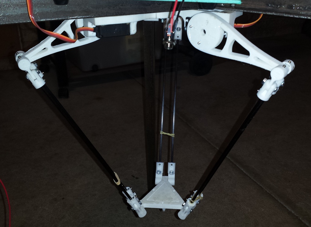
Currently, the project is operational, all parts have bfeen printed and assembled. The main controller is an Atmel ATMEGA328P micro controller which interfaces
via I2C with a PCA9685 PWM controller to set servo positions. Positional data is sent to the controller via a BC417 bluetooth module.
A Windows based control program has been written in C++/CLI.
The Windows control program is currently under development, however you may download the Visual Studio project here:
 DeltaControl.rar
The ATmega328P control program AVR Studio project can be downloaded from here:
Currently, smooth fluid motion is not achieved. This is due to lack of control that can be obtained over these servos. When a position is set, the servos turn at their maximum speed
to the set position. No velocity and/or acceleration control is achieved. Increasing the number of discrete locations should improve this jerky motion. However as there
is some delay in data transfer between the control computer and the controller, and the controller and the PCA9685 PWM chip, there is a limit to the number of commands that may be sent.
The next version of this controller will experiment with controlling the servo positions directly via PWM on the ATMEGA chip. For this, the 328P will need to be upgraded to a 1284 as this
has four 16bit PWM pins, as opposed to two.
A hardware version in which the servos are traded out for custom servos who’s velocity and acceleration can be controlled is under consideration.
Jump to: |
Goals |
[top] |
- Design a Delta robot in which all parts can be 3D printed
- Dimensions should be approximately 1/3 that of NUWAR
- Allow for maximum control versatility, ie wireless protocols and multiple platforms
- Allow for interchangeable tips
Mechanical Design |
[top] |
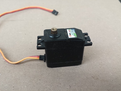 The basis of this design will be around three Power HD 1501MG servos that I have lying around. These servos are rated for 17 kg/cm, testing has shown
that a realistic stall torque varies from ~15 to ~16 kg/cm at 6V.
All parts will be 3D printed with the exception of the forearm rods; 4mm diameter carbon fibre rods will be used as forearms. I purchased these in 1 metre lengths from carbonfibre.com.au for only $5.90AUD each.
The design dimensions will be based on approximately one quarter the size of the NUWAR robot, the table below shows initial dimensions:
| Part | Length (mm) | Description |
| Lc | 100 | Length of the control arm |
| Lf | 240 + Additional length from joint | Length of the forearm. This length may vary depending on the design of the revolute joints at each end of forearm. 240mm was chosen as this divides nicely into 1 meter lengths (with 10mm overlap) |
| Re | 42 | Distance form centre of end effector to forearm joint. |
| Rb | 80 | Distance from centre of base to motor axes. |
| Lo | To be measured | The offset along the motor rotational (z) axis form the motor origin to the control arm. Due to the imperfect nature of the servo horns that will be used to connect the forearm to the servo, this may vary from servo to servo, as such, should be measured after construction. |
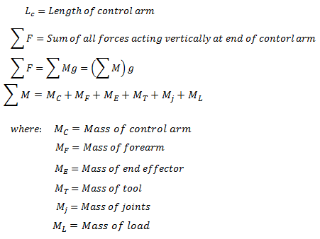
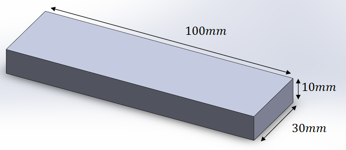
Determine Maximum Load
An approximation to the maximum load can be obtained when considering the case in which the control arm is horizontal
and all of the weight of the forearm, end effector and load is acting perpendicular to this (directly down). Also assume
that the centre of mass of the control arm is located at the end of the control arm. This allows for a generous over-estimation.
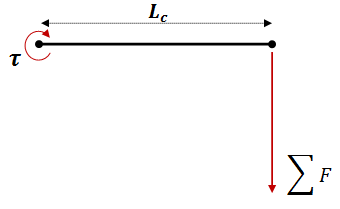
Free body diagram of maximum torque estimation
Control Arm Mass Estimate
The servo horn arms have a maximum diameter of 40mm, thus 40sin(45) = 28.2mm will be the minimum control arm height at its largest point.
Initially modelling this as a rectangular prism of length 100mm, height 30mm and width 10mm allows for a generous weight estimation which
can include less significant weight components such as the printed joints and rods/bolts used to assemble the joints.
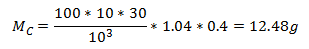
Volume estimate for control arm
The printing material, ABS, has a density of 1.04g/cm3. With a 0.4 fill density, total weight of this block will be:
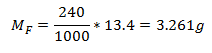
Forearm Mass
Each 1 meter carbon fibre rod weighs 13.4g:
Thus the maximum total weight of tool tip and load can be calculated:
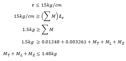
Hence the combined weight of the end effector/tool and load cannot exceed 1.48kg.
SolidWorks Design
The required parts have been designed in SolidWorks. I don’t know what I am going to do when my student licence expires. Either cry in a corner or enroll to another degree :D
Revolute Joint – 4mm diameter hole for connecting to forearm links
Download:
Revolute Joint – 2.54mm diameter hole for connecting to pin
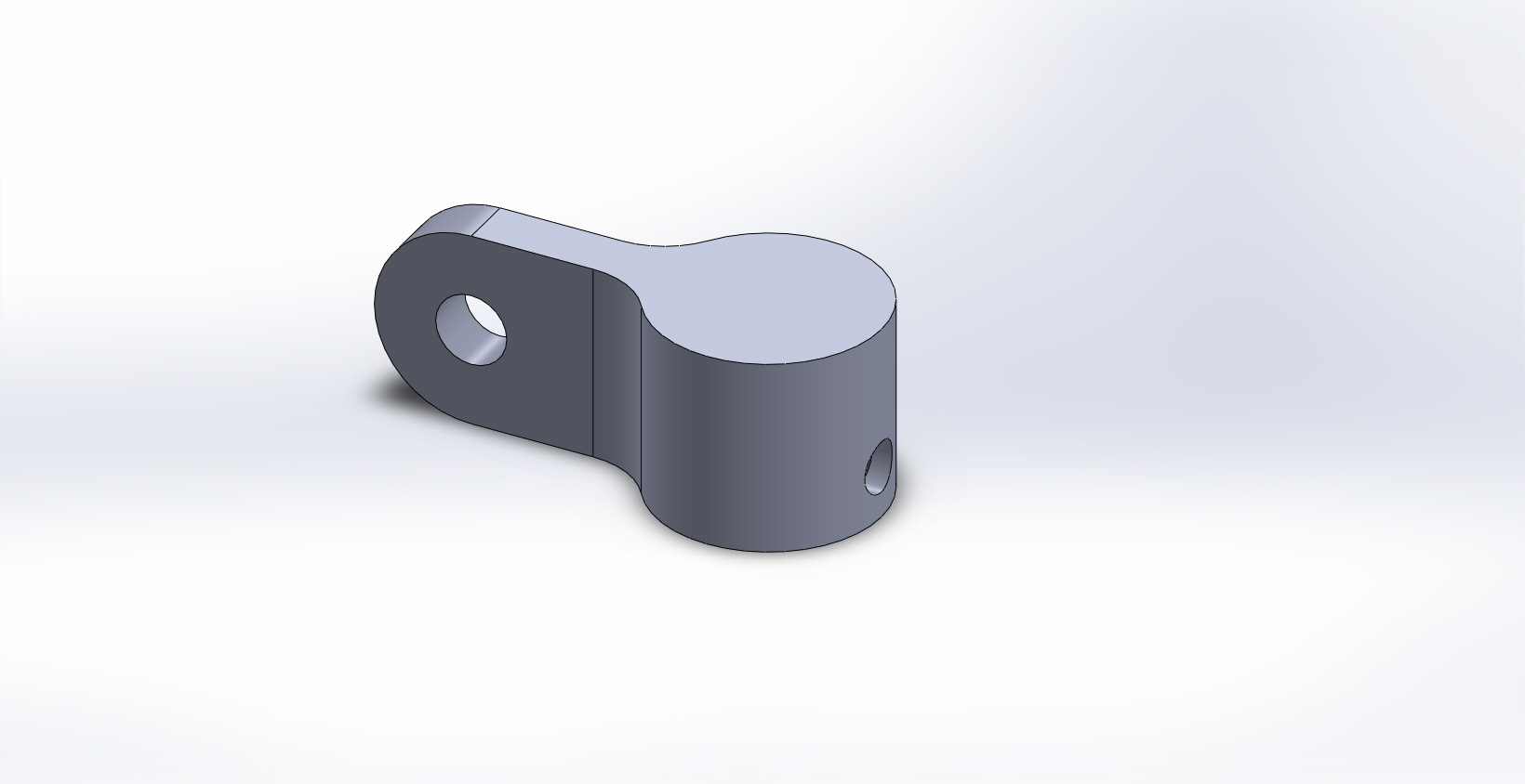
Download:
Assembly
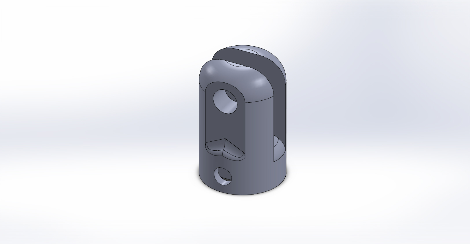
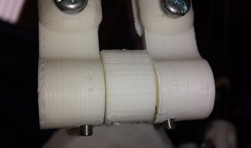
Revolute joints
The revolute joints can be connected using an m4 bolt and nut, preferably a nyloc nut to prevent loosening during operation.
An M3 grub screw is intended to securely fasten the joint to the pin/rod, an M3 size nut trap is used to hold this grub screw in place.
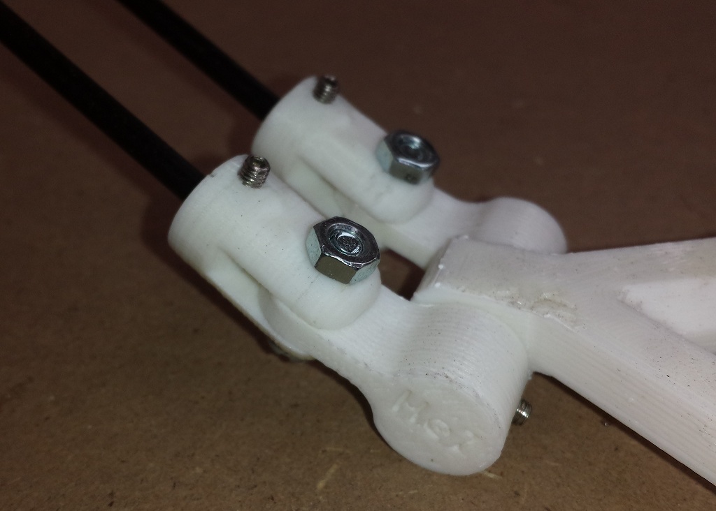
Assembled revolute joint
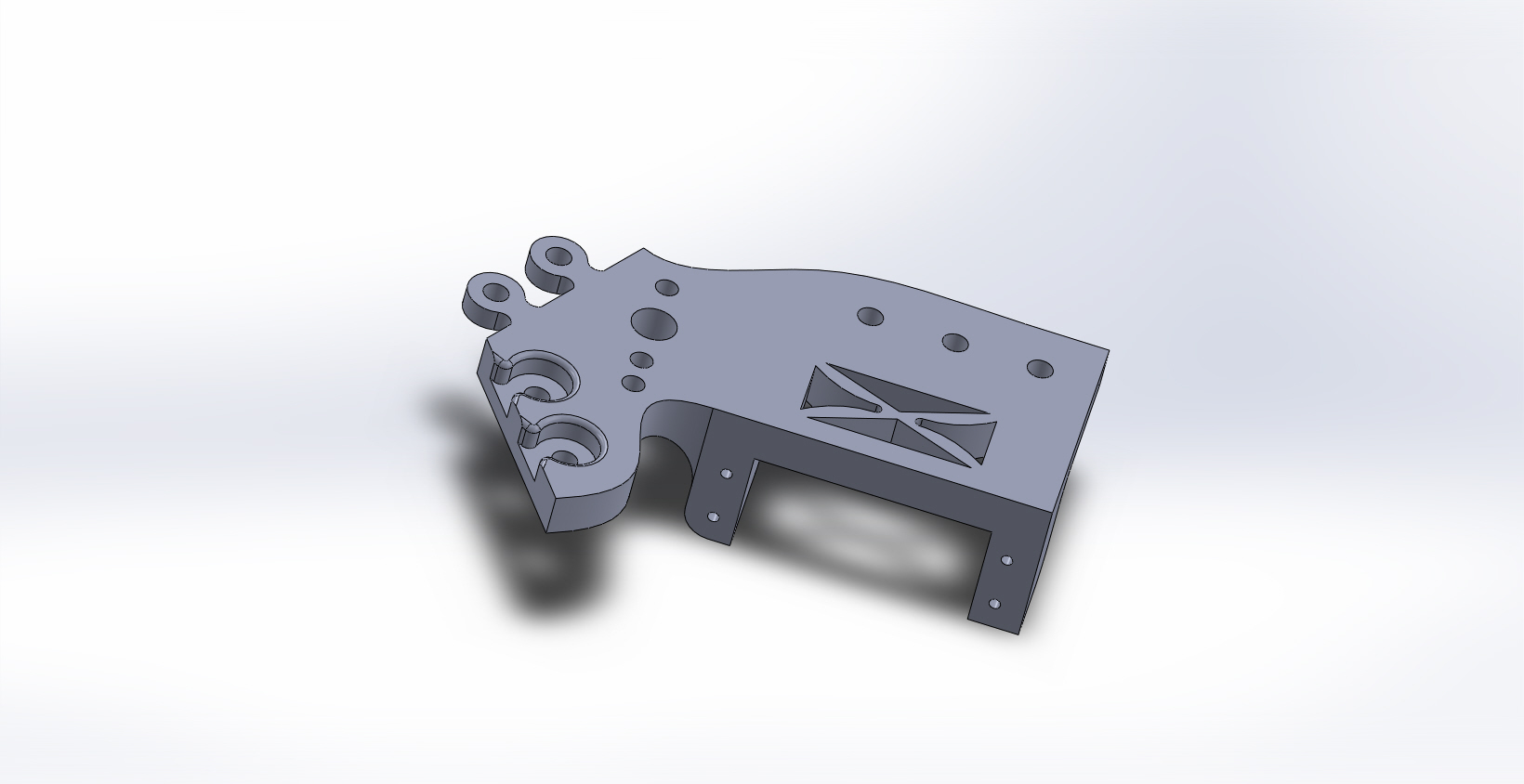
Base
The base has been designed in three identical pieces. This is to allow for smaller working area printers and to reduce the chances of warping during printing.
The tabs on each piece line up with the holes on the other, a total of six M4 bolts/nuts are used to secure the base piece together.
The mounts are designed to fit the PowerHD 1501MG servos. The servos should be installed with the motor axis farthest from the centre of the base.
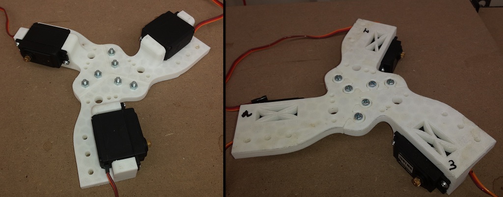
Assembled base
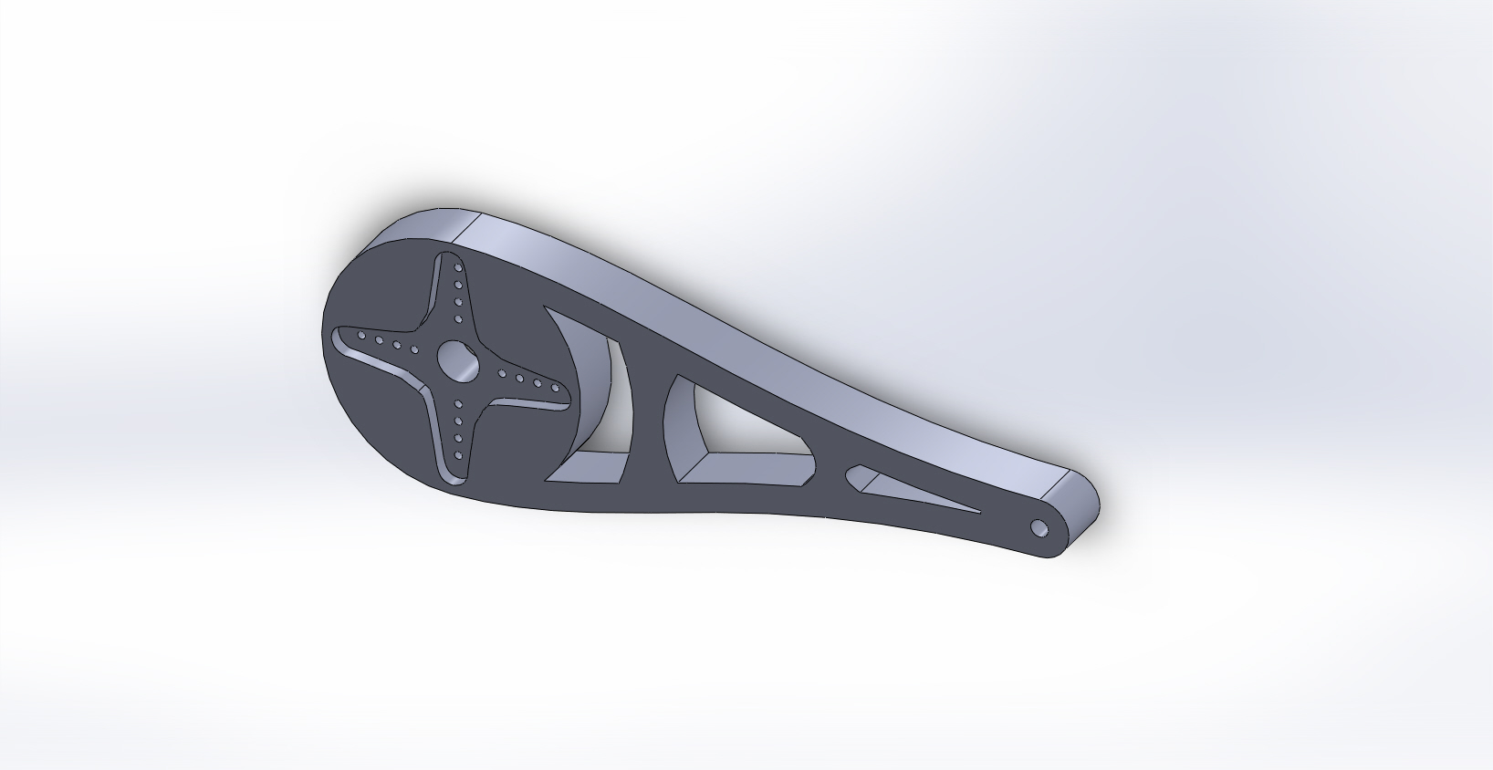
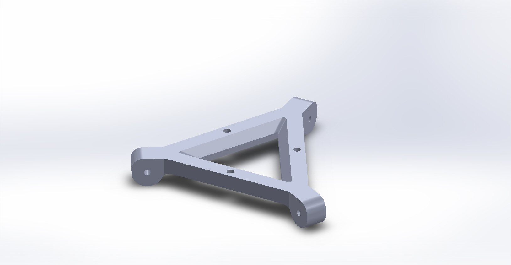
Control Arms
The control arms have a contour of the + shaped servo horn cut into it. This is the servo horn that comes with the 1501Mg servos, however
this should be a standard size. Small screws are used to attach the horn to the control arm, a hole has been left in the control arm with sufficient clearance to
screw the horn into the servo.
Once both the servo has been installed into the base, and the control arm has been installed to the servo, a set of calipers should
be used to obtain an accurate measurement of the control arm offset along the motor axis. To do this, measure the perpendicular distance between
the side face of the base and the centre of the control arm. These measurements (Lo) will be used to solve the kinematics of the robot.
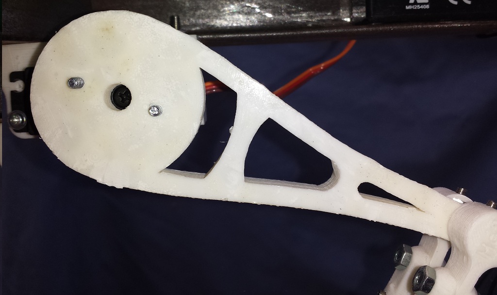
Assembled and attached control arms
Pin joints
In order to attach the revolute joints to the end effector / control arms, as well as provide the additional degree of rotational freedom at these locations, a pin joint is used.
2.54mm holes are printed into the single tab side of the revolute joints, I used the metal rod of a 2.54mm welding rod, however anything similar will do the trick.
Cut the rod to approximately 25mm in length, pass it through the hole in the end of the control arm / end effector, and secure the single tab
revolute component to each end. The original design was to use washers on either end to reduce friction, however I found this unnecessary.
Pin joints
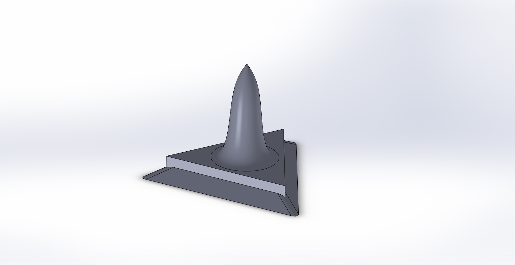
End Effector
The end effector is designed to accommodate interchangeable tips. The vertices of the inner triangle are 25mm from their centre and
there is a 45° outward draft to allow a seating for tools. Three holes can be found at the midpoint of each edge, a small tab is screwed in each hole using
an M3 bolt to secure tools in place
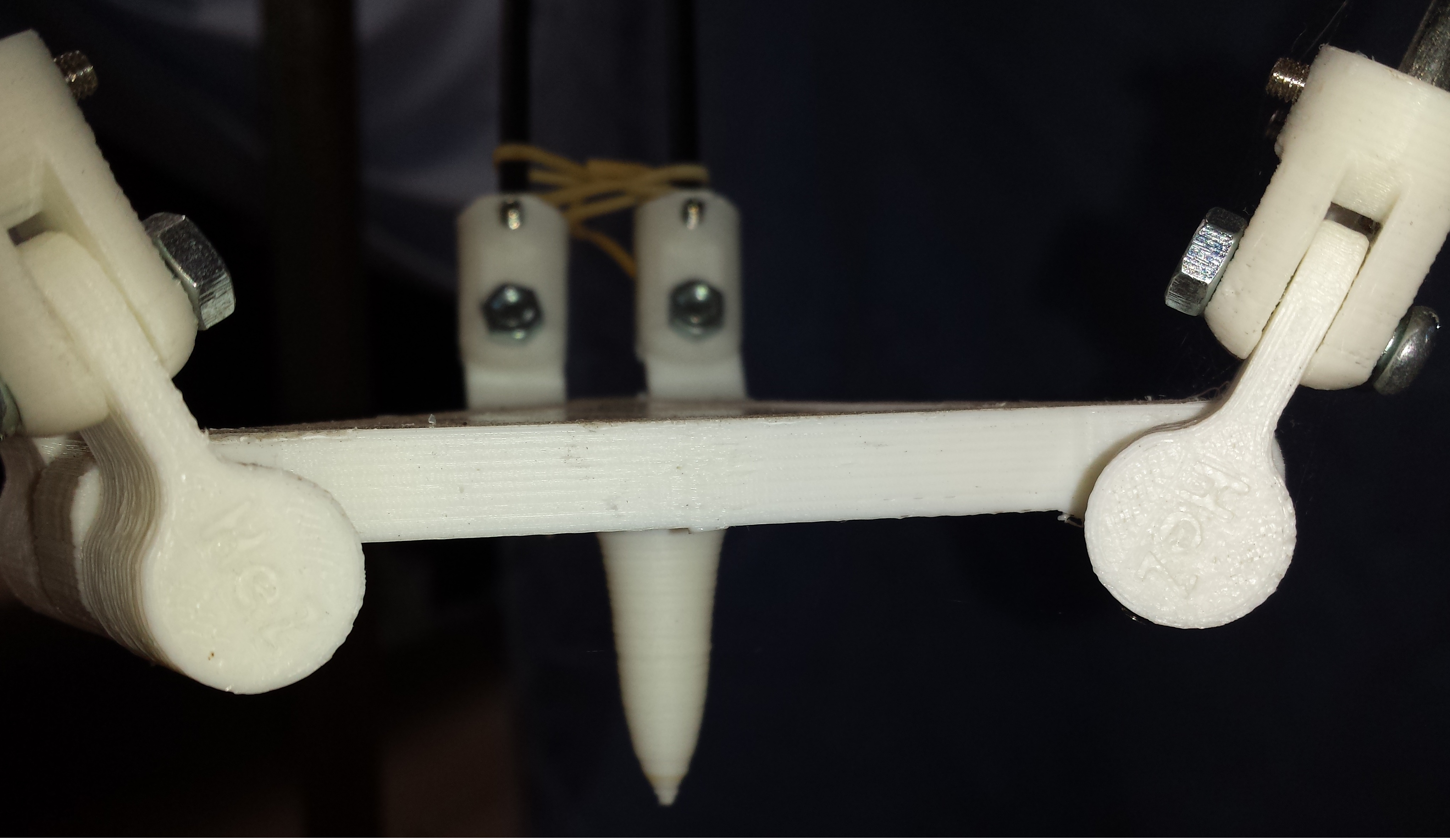
End effector with pointed tip tool
Kinematics |
[top] |
I have written programs to perform the inverse kinematics for DELTA, these are available in MATLAB or in c++
c++:
MATLAB, these use Peter Koveski’s homogeneous transform matrix functions:
Kinematics Intro
The DELAT robot is a parallel manipulator. Unlike its serial counterpart which controls the end effector using a single kinematic chain, the
parallel manipulator uses multiple kinematic chains arranged in parallel. This is advantageous as it allows the actuators to be located on an immobile base
reducing the overall weight of the links thus allowing a higher load carrying capacity; whilst also eliminating the issue of cascaded positional errors from actuators in the same kinematic chain.
Multiple links also allow the load to be distributed – increasing rigidity.
This increase in load carrying capacity and rigidity – along with several other advantages – comes at the cost of a reduces workspace volume and a lack of linearity between joint space
and task space co-ordinates.
DELTA is actuated by three motors, all of which are located on an immobile base. Each of the serial chains that connect these motors to the end effectors contains one passive joint at the elbow.
In a serial manipulator, the forward kinematics (determining the position of the end effector for known joint angles) is a trivial problem. Knowing the angles of the joints and
lengths of the links , simple geometry may be used to calculate the end effector position. However due to these passive joints, there are multiple solutions to the forward kinematic problem for DELTA.
Conversely, the inverse kinematics problem (determining the joint space co-ordinates to achieve a task space position) is non trivial for a serial manipulator as there are multiple
arrangements of joints that can result in the same end effector position; it is trivial for the parallel manipulator. This is fortunate for this project as we are interested in controlling the
end effector location of DELTA by actuating its motors.
DELTA Inverse Kinematics
The first step in the kinematic analysis is to define some co-ordinate systems. First we need a base co-ordinate system. The base co-ordinate system will be used to define
the position of the end effector. We also need a joint space co-ordinate system – a co-ordinate system to define the position of each of our motors. Finally a motor co-ordinate system is required to describe the position of the
end effector relative to the motor.
First consider a motor, we can apply a Cartesian co-ordinate system to this motor, call it [xyz], in which the rotational axis of the motor is aligned along the z axis.
The arm will rotate in the xy plane, I define the rotation vector as positive in the positive z direction, so rotation is positive from x to y. This is the
motor co-ordinate system and each motor has one. It is using this co-ordinate system that the angle of each motor will be calculated (the angle between the control arm and the
motor x axis).
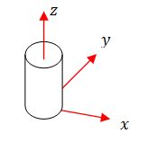
Motor Co-ordinate system [xyz]
Now consider the triangular plane created by placing the vertices of a triangle on the rotational axis of each of the three motors; where the centreline of the triangle is perpendicular to the rotational axis.
This will be the base plane and the origin of the base co-ordinate system [XYZ] will be located at the centre of this triangle. Positive Z is defined as pointing ‘up’ or away from the
robot workspace. Positive X is coincident with the line perpendicular to motor 1 rotational axis and intersecting the triangle centre.
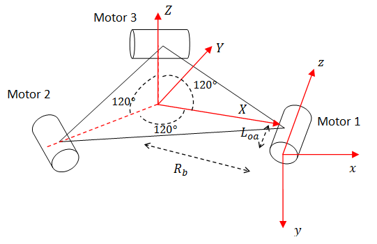
Base and motor co-ordinates
As we will know a position in base co-ordinates and are required to calculate the corresponding motor angles, it is necessary to convert a point in base co-ordinates [XYZ] to motor co-ordinates [zyx].
A Denavit–Hartenberg transform will be used to align the base co-ordinates
with the motor co-ordinates in order to provide a transform matrix to convert an end effector position in base co-ordinates to motor co-ordinates.
I have defined that a positive motor rotation should be “downward”, that is, zero degrees makes the control arm parallel with the base plane and a positive angular displacement will
cause the arm to rotate down towards the workspace. As depicted in the figure above, this required the motor to be rotated -90 degrees about the X axis, then translated a distance Rb
along X. The D-H parameters are as follows:
| Parameter | Value | Description |
| theta | 0 | Rotation required to align old and new x axis |
| d | 0 | Depth along previous z axis, from origin to common normal |
| r | Rb | Length of common normal |
| alpha | -90 deg | Rotation about new x axis to put z in line with joint motion. |
The resulting homogeneous transform matrix:
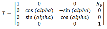
A further shift of -Loi along the motor z axis will be used to shift the origin to the centre of the control arm for each motor. Each motor will have a different offset here
due to the nature of the servo horns used to connect the arm to the servo. Each one has a different fit.
Motors two and three are pre-multiplied by a homogeneous rotation matrix in order to rotate the base co-ordinates about the z axis before translating. This allows the motors to be placed
on a triangle 120 degrees apart. Sample MATLAB code is shown below to illustrate the matrix multiplication required:
|
1 2 3 4 |
motorAxes = dhtrans(0, 0, Rb-Re, -pi/2); % The general motor axes motor1 = motorAxes * trans(0, 0, -Lo(1)); motor2 = rotz(2*pi/3) * motorAxes * trans(0, 0, -Lo(2)); motor3 = rotz(4*pi/3) * motorAxes * trans(0, 0, -Lo(3)); |
Here, the length of the common normal in the D-H transform is defined as the length Rb – Re in order to simplify later calculations.
These transform matrices motor1, motor2 and motor3 convert a point in motor co-ordinates to a point in base co-ordinates;
|
1 |
P = motor1 * P_motor1; |
However it is required to obtain the point in motor co-ordinates using the known point in base co-ordinates. The inverse of the motor transform matrices is required.
When taking this inverse, care is taken to preserve the augmented homogeneous dimensions.
The position of the end effector location is now known in each of the motor co-ordinates systems. The angle required to position the arm and achieve this end effector location
can now be calculated for each motor independently using some geometry:
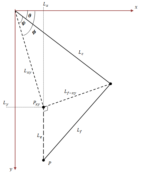
Geometry of an arm
Hence we can calculate θ by:

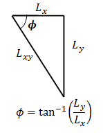
Calculate φ
φ can be easily calculated by considering the projection of the point P onto the xy plane of the motor axis:
Calculate ψ
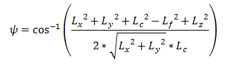
ψ is a little bit trickier to calculate however the same complexity of geometry is used. ψ is the internal angle of a triangle in which all
three sides can be calculated, the cosine rule is applied:
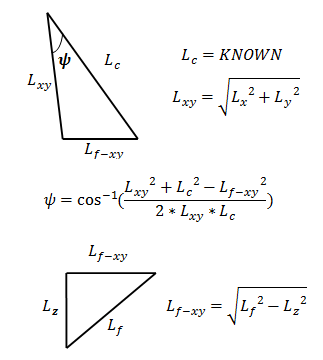
Expressing ψ in terms of known values:
And finally we have the solution to θ for this motor:
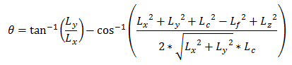
NOTE: A four quadrant inverse tan calculation should be used for calculation of φ to ensure the correct sign.
NOTE2: A check should be made to ensure that an end effector location is in fact within the workspace. If using my kinematic functions,
the programs will allow calculation of an impossible configuration, however will return a dummy result. (A complex number will be returned in MATLAB code,
a NaN will be returned in the c++ code).
Controller |
[top] |
In the interest of maximizing control versatility, the controller used will be an ATMEL 8bit micro controller.
A set of serial commands will be used to communicate with the controller and instruct the robot. The servo PWM signals are
controlled via a PCA9685 12-bit PWM I2C controlled LED driver. This is designed to drive 16 channels of LEDs, however as
it has a high (12-bit) resolution and can maintain a steady clock 50Hz clock from its internal oscillator, it is suitable to reliably drive
these analog servos.
I have written a simple driver to communicate with the PCA9685 via an AVR ATMega series micro controller, along with a simple master transmit
I2C algorithm. This code should be portable across all ATMega series with minimal I/O tweaking.
PCA9685 Driver
Download:
The AVR controller accepts serial commands over UART, only valid commands will be accepted. A particular sequence of valid ASCII characters is expected, depending on the command set.
| Command | Expected Value | Description |
| A | A<sign>##### | Move motor A to absolute position. After transmitting an ASCII A character, an ASCII + or – is expected, followed by 5 ASCII characters 0-9. These numbers represent an absolute angle to turn the servo to to two significant figures (000.00 to 360.00) |
| B | B<sign>##### | LMove motor B to absolute position. After transmitting an ASCII A character, an ASCII + or – is expected, followed by 5 ASCII characters 0-9. These numbers represent an absolute angle to turn the servo to to two significant figures (000.00 to 360.00) |
| C | C<sign>##### | Move motor C to absolute position. After transmitting an ASCII A character, an ASCII + or – is expected, followed by 5 ASCII characters 0-9. These numbers represent an absolute angle to turn the servo to to two significant figures (000.00 to 360.00) |
| D | D<sign>############### | Move motor A, B and C to absolute position. After transmitting an ASCII A character, an ASCII + or – is expected, followed by 15 ASCII characters 0-9. These numbers represent an absolute angle to turn the servo to to two significant figures (000.00 to 360.00). the first 5 characters are servo A, second 5 are B and final 5 are C |
NOTE: Future versions will eliminate the sign character requirement. This was originally used for relative movement, however relative
movement is taken care of at client end now.
UART Communication Protocol and Motor Controller
Download:
Servo Angle/Duty Cycle Relation
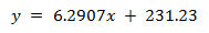
In order to set the servo to a desired angle, the relationship between servo angle and servo PWM duty cycle needs to be determined. By measuring the angle
at a collection of duty cycles, linear regression is used to determine the relationship:
| Pulse Width (ms) | Angle(deg) | Angle(deg) | Angle(deg) | Angle(deg) |
| 300 | 9 | 9 | 8 | 8.67 |
| 400 | 26 | 26 | 26 | 26 |
| 500 | 44 | 43 | 42 | 43 |
| 600 | 59 | 59 | 59 | 58.67 |
| 700 | 76 | 75 | 76 | 75.67 |
| 800 | 91 | 92 | 92 | 91.67 |
| 900 | 109 | 108 | 108 | 108.33 |
| 1000 | 123 | 122 | 122 | 122.33 |
| 1100 | 139 | 137 | 137 | 137.67 |
| 1200 | 153 | 151 | 152 | 152 |
| 1300 | 170 | 169 | 169 | 169.33 |
| 1400 | 185 | 186 | 185 | 185.33 |
These values are consistent for all three servos that I have. However may vary from servo to servo
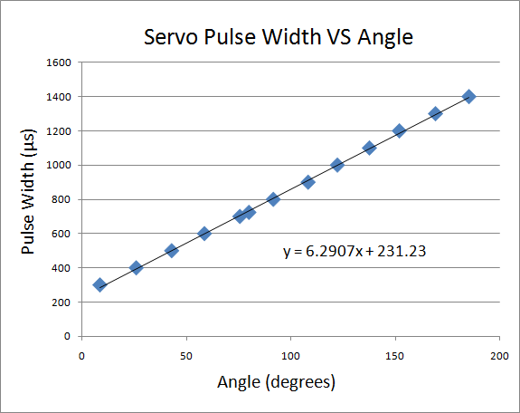
A strong linear relation can be seen here, as such linear regression is suitable to determine an equation relating pulse width to angle:
Electrical Design |
[top] |
The electrical design is still being finalized, The EagleCad board has been sent away for manufacture and I will release this after it has been assembled and tested
Control Program |
[top] |
The control program is currently under beta development, however you may download the project here:
A Windows based control program has been designed in C++/CLI, this program incorporates the inverse kinematics to allow robot position to be set
in either joint space or task space:
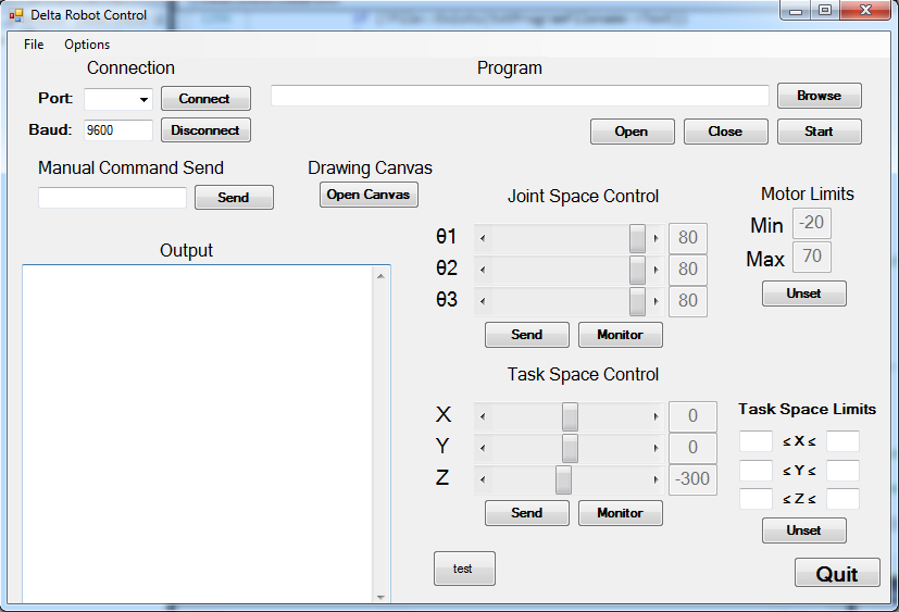
Delta Robot control program
The control program has five modes in which it can operate. The default mode is “send” mode. In this mode, a custom command string may be sent
to the controller, or the sliders can be used to set the axis in either joint space or task space to the desired value and sent to the controller using the respective send button.
The joint space and task space sliders each have their own monitor button, pressing this will enter “monitor” mode for that co-ordinate system. In
monitor mode, commands will be continuously sent to the robot allowing it to track the position of the slider in real time.
The fourth mode is “program mode. In program mode, a properly formatted tab or white space delimited .txt file which represents a motion program is uploaded. This file consists of a header section
followed by a data section. The header section describes the program characteristics and the data section contains the position in the selected co-ordinate system. Each line represents a
different discrete time.
Program Header
|
1 |
Co-ordinate system defines what the co-ordinates in the proceeding section represent, they may be;
- JS
- TS
- BC
Where JS represents Joint Space, TS represents Task Space, and BC represents Base co-ordinates. For current purposes, BC and TS are the same, however it is included for completeness.
Sample Time represents the delay between each of the co-ordinates in milliseconds.
Interpolation type indicates how the controller should handle moving between each of these discrete positions in joint space. Currently only linear interpolation is implemented in the controller.
ie. The servos are actuated from position A to position B at maximum speed
Example code for a circle in the xy plane:
|
1 2 3 4 5 6 7 8 9 10 11 12 13 14 15 16 17 18 19 20 |
BC 50.0000 Linear 0.000 80.000 -300.000 26.176 75.597 -300.000 49.470 62.871 -300.000 67.318 43.224 -300.000 77.755 18.819 -300.000 79.633 -7.658 -300.000 72.744 -33.292 -300.000 57.847 -55.261 -300.000 36.582 -71.146 -300.000 11.290 -79.199 -300.000 -15.245 -78.534 -300.000 -40.102 -69.223 -300.000 -60.544 -52.291 -300.000 -74.321 -29.603 -300.000 -79.916 -3.657 -300.000 -76.714 22.693 -300.000 -65.066 46.544 -300.000 -46.256 65.272 -300.000 -22.353 76.814 -300.000 |
The final mode is “canvas” mode. This is a drawing canvas which tracks the position of the cursor along the canvas.
A pen mount tool is currently being designed which will allow the robot to hold a pen, and draw whatever the user draws on the canvas.
When the mouse button is not pressed, the end effector position will track the position of the cursor on the canvas in the XY plane at a height of z max.
When the mouse is held, the pen will draw on the canvas and the z position of the XY plane will move down to z min. Hence when drawing on the canvas, the robot
will also draw on an appropriately positioned drawing plane.
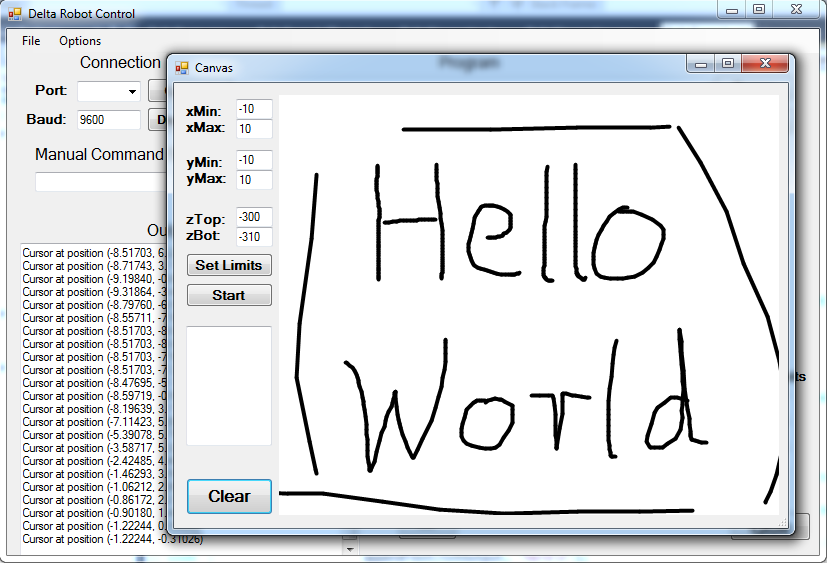
Canvas Draft
Hi
Problem link (Control Program)
Tankx
Thanks!
All Fixed.
HI, i like your work.. . i want to make a delta robot as final year project, if i need to move a load of approx 1 kg with robot, what minimum dimensions will be required.
There aren’t necessarily any minimum dimensions required to move a load. It really depends on the amount of torque that you motors can provide. A good way to get a ballpark figure of the torque that your motors will need to provide is to multiply the 1kg by the length of your upper arm (that will give the torque for when the arm is fully extended horizontally and the load is directly under it. It also assumes that all of the load is supported by that one arm – which is of course not the case for a parallel manipulator).
So the smaller the robot the easier it will carry the load. There is no minimum dimensions from a load carrying perspective, only from a practicality perspective – ie how far the load needs to be moved and how fast.
However if this is your final year project you will likely need to do a lot of research into the dynamics of moving a 1kg load before you even start to think about what dimensions your arms will be. Delta robots are known for their actuation speed and acceleration, so for a 1kg load you will need to consider the inertia involved to start/stop and follow trajectories. The inertia will likely contribute to higher forces on the motors than just lifting the load.
There are a great deal of papers out there that have already done very in depth analysis of this. I know because I have read many of them. If you are doing this for a final year project, you will need to spend the first couple months on a literature review anyway so by the time you are finished with that, you can probably tell me more about delta dynamics.
This is awesome! I was trying to apply your code to my robot, I will only have to modify de geometry, right? What’s the origin or home coordinates of the robot? (X=0, Y=0, Z=0) ?
Hi Rafael,
Provided that you have the same controller (PCA9685), you should just be able to change the geometries and away you go. If you have a different controller then it is unlikely that the serial commands will be compatible – you will need to change those too.
Home is at the center of the base of the robot – this is a point in the same plane as the motors and at an equal distance from all motors. X points towards motor 1, Z points upwards and Y is mutually orthogonal. It is depicted here:

Ah ok. Thanks for your answer. I have only 2 more questions.
– If I get a theta = 0 that will mean the control arm will be horizontal?
– The theta angles are positive – CW right ?
Thanks a lot.